#Read the penguines_sampl data off GITHubpenguins<-read_csv("https://raw.githubusercontent.com/mcduryea/Intro-to-Bioinformatics/main/data/penguins_samp1.csv")
Rows: 44 Columns: 8
── Column specification ────────────────────────────────────────────────────────
Delimiter: ","
chr (3): species, island, sex
dbl (5): bill_length_mm, bill_depth_mm, flipper_length_mm, body_mass_g, year

ℹ Use `spec()` to retrieve the full column specification for this data.
ℹ Specify the column types or set `show_col_types = FALSE` to quiet this message.
#See the first six rows of data added to notebookpenguins %>%head()
# A tibble: 6 × 8
species island bill_length_mm bill_depth_mm flipper_leng…¹ body_…² sex year
<chr> <chr> <dbl> <dbl> <dbl> <dbl> <chr> <dbl>
1 Gentoo Biscoe 59.6 17 230 6050 male 2007
2 Gentoo Biscoe 48.6 16 230 5800 male 2008
3 Gentoo Biscoe 52.1 17 230 5550 male 2009
4 Gentoo Biscoe 51.5 16.3 230 5500 male 2009
5 Gentoo Biscoe 55.1 16 230 5850 male 2009
6 Gentoo Biscoe 49.8 15.9 229 5950 male 2009
# … with abbreviated variable names ¹flipper_length_mm, ²body_mass_g
A data set containing general characteristics from a sample of the Gentoo penguin population on Biscoe Island.
Data Manipulation
This section covers techniques for filtering rows, subsetting columns, grouping data, and computing summary statistics in R. Filtering rows allows you to select only those rows that meet certain criteria, while subsetting columns allows you to select only a subset of the available columns. R allows for these functions, as well as dividing the data set into groups based on common characteristics that can create new ways of interpreting information. Using Computing to create summary statistics involves calculating statistical measures such as mean, median, and standard deviation for each group. Understanding how to use R to accomplish this analysis is crucial for grouping and summarizing large quantities of data, which can be combined to answer complex questions about the whole set.
Questions to consider about Penguins
How does the body mass of different penguin species compare?
What is the distribution of beak length and depth among penguin species?
How does flipper size vary among different penguin species?
Is there a correlation between flipper size and body mass in penguins?
How does flipper size vary within a single penguin species over time?
How does flipper size differ between male and female penguins of the same species?
How does flipper size relate to the preferred habitat of a penguin species (is it larger in species that inhabit colder environments)?
library(kableExtra)
Attaching package: 'kableExtra'
The following object is masked from 'package:dplyr':

    group_rows
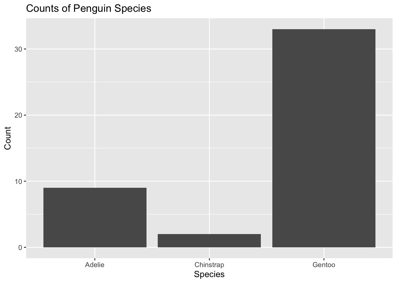
penguins %>%ggplot() +geom_bar(mapping =aes(x = species)) +labs(title ="Counts of Penguin Species",x ="Species", y ="Count")
Single-Numerical Variable using histograms
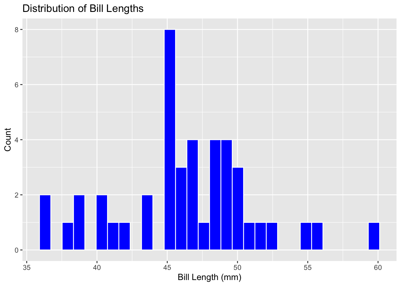
penguins %>%ggplot() +geom_histogram(mapping =aes(x = bill_length_mm),color ="white",fill ="blue") +labs(title ="Distribution of Bill Lengths",x ="Bill Length (mm)", y ="Count")
`stat_bin()` using `bins = 30`. Pick better value with `binwidth`.
Two-Variable Numerical Analysis
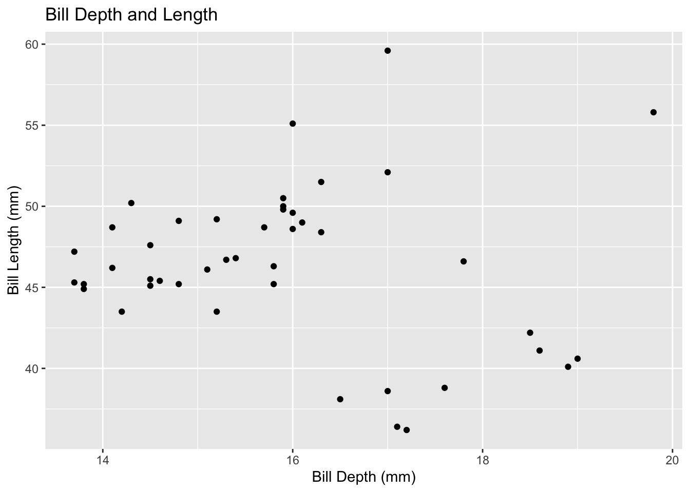
penguins %>%ggplot() +geom_point(mapping =aes(x = bill_depth_mm, y = bill_length_mm)) +labs(title ="Bill Depth and Length",x ="Bill Depth (mm)",y ="Bill Length (mm)")
Bill size seems to average around the 45-50mm length and 14-16mm depth.
Some outlying data in this set were around 40mm length and 17-18mm length
Two-Variable Categorical Analysis
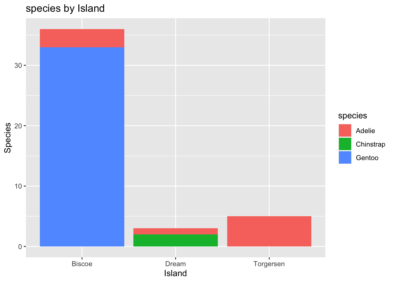
penguins %>%ggplot() +geom_bar(mapping =aes(x = island, fill = species)) +labs(title ="species by Island",x ="Island",y ="Species")
conclusions:
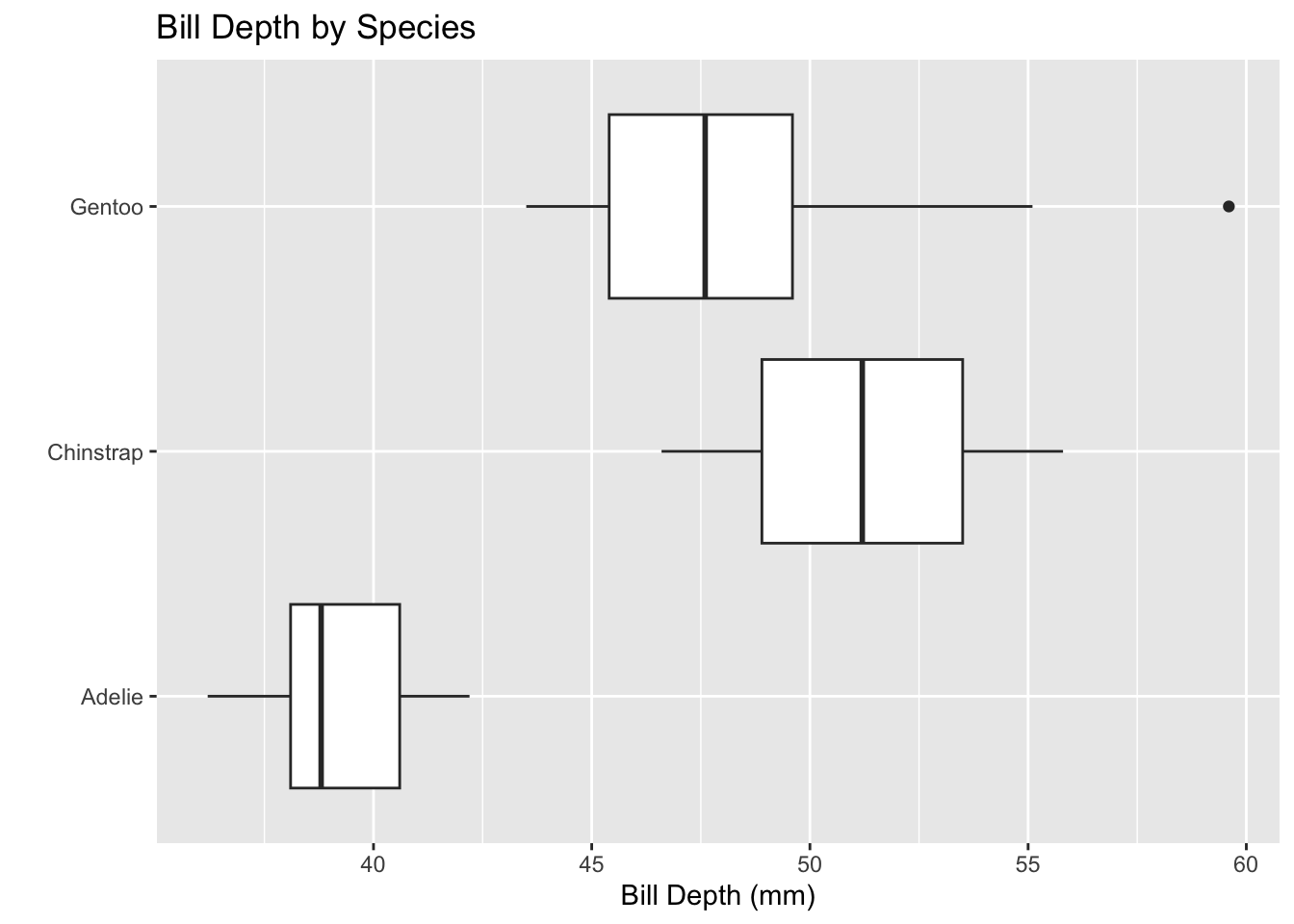
Numerical & Categorical Comparison: Boxplots
penguins %>%ggplot() +geom_boxplot(mapping =aes(x = bill_length_mm, y = species)) +labs(title ="Bill Depth by Species",x ="Bill Depth (mm)",y ="")
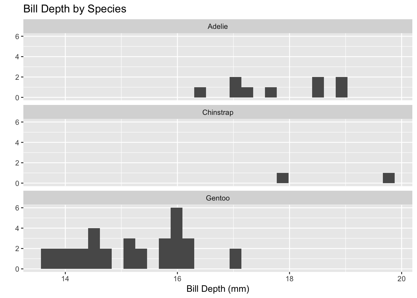
Numerical & Categorical Comparison: Faceted Plots
penguins %>%ggplot() +geom_histogram(mapping =aes(x = bill_depth_mm)) +facet_wrap(~species, ncol =1) +# 'facet' is group of variables or expressions within the aes. 'wrap' allows for alterations of the col (ncol) and line (nrow) labs(title ="Bill Depth by Species",x ="Bill Depth (mm)",y ="" )
`stat_bin()` using `bins = 30`. Pick better value with `binwidth`.
Conclusions:
Advanced Plotting
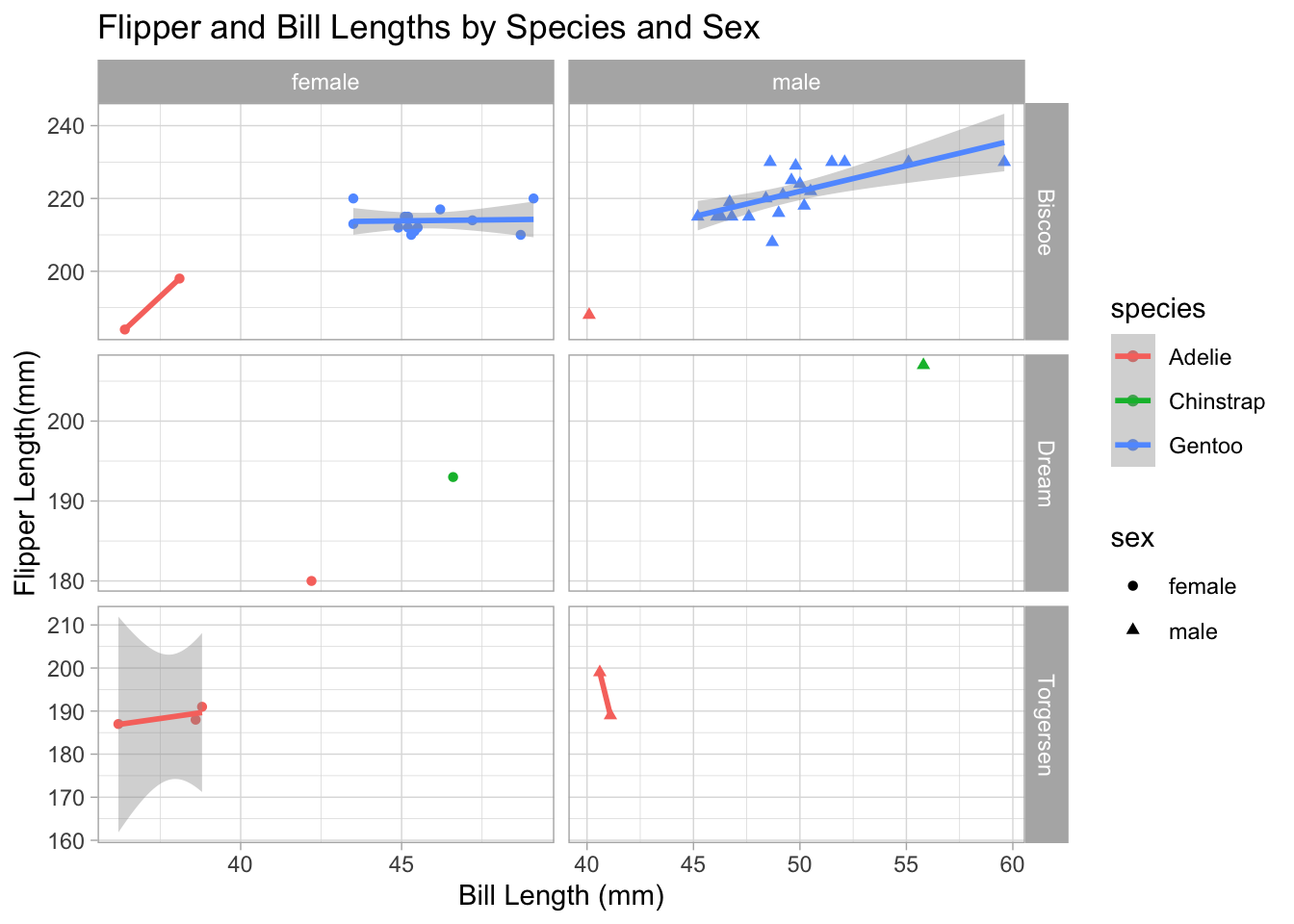
Two Continuous-Variable Comparison
works with both numerical and categorical variables
“continuous” may be one, or both of the variables
penguins %>%filter(!is.na(sex)) %>%ggplot() +geom_point(mapping =aes(x = bill_length_mm, y = flipper_length_mm,color = species,shape = sex)) +# geom_point = SCATTERPLOT; useful for numerical, categorical, or combined comparisons. geom_smooth(mapping =aes(x = bill_length_mm,y = flipper_length_mm,color = species),method ="lm") +# 'smooth' reduces the visual complexity of the geom (graph), can be altered in many different ways.facet_grid(island ~ sex, scales ="free") +labs(title ="Flipper and Bill Lengths by Species and Sex",x ="Bill Length (mm)",y ="Flipper Length(mm)") +theme_light()
`geom_smooth()` using formula = 'y ~ x'
Warning in qt((1 - level)/2, df): NaNs produced

Warning in qt((1 - level)/2, df): NaNs produced
Warning in max(ids, na.rm = TRUE): no non-missing arguments to max; returning
-Inf

Warning in max(ids, na.rm = TRUE): no non-missing arguments to max; returning
-Inf