Attaching package: 'dplyr'The following objects are masked from 'package:stats':
filter, lagThe following objects are masked from 'package:base':
intersect, setdiff, setequal, union
Attaching package: 'dplyr'The following objects are masked from 'package:stats':
filter, lagThe following objects are masked from 'package:base':
intersect, setdiff, setequal, uniondatum <- read_csv("C:/School/23SPDAY/FieldMethodsandTech/Practice Data/linear regression/anova/Class Activity 9.csv",
show_col_types = FALSE)
names(datum)[names(datum) == "Land use"] <- "land_use"
list(datum)[[1]]
# A tibble: 44 × 2
land_use Nitrogen
<chr> <dbl>
1 Agriculture 0.986
2 Agriculture 1.03
3 Agriculture 1.10
4 Agriculture 0.921
5 Agriculture 0.976
6 Agriculture 0.976
7 Agriculture 1.03
8 Agriculture 0.951
9 Agriculture 1.13
10 Agriculture 0.974
# … with 34 more rowsANOVA (Analysis of Variance) is a statistical technique used to compare means between three or more groups.
ANOVA tests whether the differences between group means are statistically significant or simply due to chance.
The basic idea behind ANOVA is to partition the total variability in a dataset into two parts: variability between groups and variability within groups.
F- Values describe the ratio of the variance between groups to the variance within groups. It indicates the degree of variation in the dependent variable (in this case, the amount of nitrogen generated) that is explained by the independent variable (in this case, the land use types).
summary(datum) land_use Nitrogen
Length:44 Min. :0.6585
Class :character 1st Qu.:0.8988
Mode :character Median :1.0152
Mean :1.1115
3rd Qu.:1.3757
Max. :1.6658 datum %>%
ggplot(aes(x = land_use, y = Nitrogen, fill = land_use)) +
geom_boxplot() +
labs(x = "Land Use", y = "Nitrogen", title = "Nitrogen by Land Use") +
scale_fill_manual(values = c("Agriculture" = "lightblue", "Forest" = "darkgreen", "Developed" = "gray")) +
theme_classic()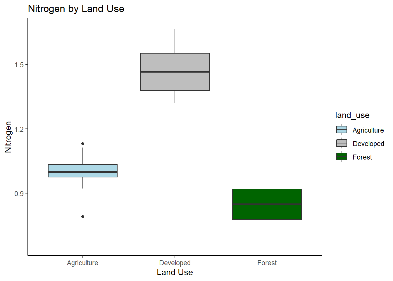
This graph suggests that land use for developement as a source of nitrogen seems to be significantly greater then both agriculture and forest. It also seems that the relationship between forest and agriculture is also significant.
results = aov(Nitrogen~as.factor(land_use), data= datum)

summary(results)
Df Sum Sq Mean Sq F value Pr(>F)
as.factor(land_use) 2 3.242 1.6210 153.6 <2e-16 ***
Residuals 41 0.433 0.0106
---
Signif. codes: 0 '***' 0.001 '**' 0.01 '*' 0.05 '.' 0.1 ' ' 1TukeyHSD(results) Tukey multiple comparisons of means
95% family-wise confidence level
Fit: aov(formula = Nitrogen ~ as.factor(land_use), data = datum)
$`as.factor(land_use)`
diff lwr upr p adj
Developed-Agriculture 0.4780560 0.3852349 0.57087717 0.0000000
Forest-Agriculture -0.1533935 -0.2462146 -0.06057233 0.0007017
Forest-Developed -0.6314495 -0.7226562 -0.54024275 0.0000000The ANOVA test showed a significant difference in the mean amount of nitrogen generated between land uses (developed, agriculture, and forest) with a large F-value (153.6) suggesting a much greater variation between groups, then within them. and a p-value < 0.05. The Tukey post-hoc analysis revealed that the mean amount of nitrogen generated in developed land use (mean = 2.74) was significantly higher than that of agriculture (mean = 2.26) and forest (mean = 2.59) land use with p-values < 0.001 and < 0.0001, respectively. On the other hand, the mean amount of nitrogen generated in forest land use was significantly lower than that of developed and agriculture land use with p-values < 0.0001 and 0.0007, respectively. However, there was no significant difference in the mean amount of nitrogen generated between agriculture and forest land use (p = 0.70).